Simulation of the 3/2 model using the Quadratic exponential scheme#
In order to achieve maximum performance of Pytorch in a Monte-Carlo simulation it is critical to vectorize over the number of simulations. Thus we need to remove all ‘if’ statements from the Quadratic Exponential scheme. Here we are also comparing the numerical performance with a standard Milstein-Euler scheme
[10]:
#import torch
import numpy as np
from quant_analytics_torch.analytics import blackanalytics
from icecream import ic
from quant_analytics_torch.calculators.multivariatebrownianbridge import MultivariateBrownianBridge
from quant_analytics_torch.analytics.norminv import norminv
import matplotlib
from matplotlib import pyplot as plt
from quant_analytics_torch.analytics import maxsoft
from quant_analytics_torch.analytics.characteristicfunction import heston_option_price, threeovertwo_option_price
[11]:
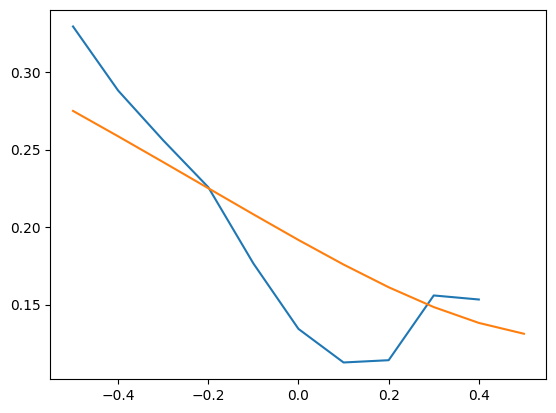
strikes = [-0.5, -0.4, -0.3, -0.2, -0.1, 0, 0.1, 0.2, 0.3, 0.4, 0.5]
ivs_heston = []
ivs_3_2 = []

for it in strikes:
    strike = np.exp(it)
    price = heston_option_price(strike,1,0.04,1,0.04,1,-0.7,1)
    iv = blackanalytics.impliedvolatility(price,1,strike,1)
    ivs_heston.append(iv)

for it in strikes:
    strike = np.exp(it)
    price = threeovertwo_option_price(strike,1,0.04,22,0.09,8,-0.8,1)
    iv = blackanalytics.impliedvolatility(price.real,1,strike,1)
    ivs_3_2.append(iv)

print(ivs_heston)
print(ivs_3_2)
[0.329324589130455, 0.28804817090987134, 0.2559429643335339, 0.22570594900838947, 0.1765775635550539, 0.13437616926929888, 0.11274163089679885, 0.11420776457099098, 0.15594420454274932, 0.1533360730988036, inf]
[0.27490070281895745, 0.2585383473876623, 0.24188987704203105, 0.22506545950438872, 0.208247085020842, 0.19171477686187532, 0.17586904342594117, 0.16123827628813256, 0.14846157304813323, 0.13824363532984824, 0.13125438320876792]
[9]:
plt.plot(strikes,ivs_heston)
plt.plot(strikes,ivs_3_2)
[9]:
[<matplotlib.lines.Line2D at 0x7fe263369e90>]
[2]:
def milstein_euler_simulation(rho, theta, kappa, eta, T, paths, n_dt):
    dt = T/n_dt
    dim = n_dt
    sobol_engine =  torch.quasirandom.SobolEngine(2*dim)
    x = sobol_engine.draw(1)
    u = sobol_engine.draw(paths,dtype=torch.float64)

    states = 2
    dim = n_dt

    fm = torch.zeros(size=(states,states))

    fm[0][0] = 1.
    fm[0][1] = 0.
    fm[1][0] = 0.
    fm[1][1] = 1.
    fwd_cov = torch.zeros(size=(dim, states, states))

    for i in range(dim):
        fwd_cov[i] = fm

    multivariate_brownian = MultivariateBrownianBridge(fwd_cov)

    y = norminv(u)
    y = torch.reshape(y, shape=(dim,states,paths))

    dz = multivariate_brownian.path(y, True)

    X = torch.zeros([paths])
    V = torch.zeros([n_dt+1,paths])
    Vt = torch.zeros([paths])
    Vt[:] = theta
    V[0] = theta

    for i in range(n_dt):
        z2 = dz[i][1]
        z1 = dz[i][0]
        Vt = torch.maximum((Vt + kappa*theta*dt + eta*torch.sqrt(Vt*dt)*z2+0.25*eta*eta*dt*(z2*z2-1.))/(1+kappa*dt),torch.tensor(0.))
        X = X - V[i]*dt/2 + torch.sqrt(V[i]*dt)*(rho*z2 + torch.sqrt(1-rho*rho)*z1)
        V[i+1] = Vt
    return X
[3]:
def quadratic_exponential(rho, theta, kappa, eta, T, paths, n_dt):
    dt = T/n_dt
    dim = n_dt

    gamma1 = 0.5
    gamma2 = 0.5

    K0 = -(rho*kappa*theta)*dt/eta
    K1 = gamma1*dt*(-0.5+(kappa*rho/eta))-(rho/eta)
    K2 = gamma2*dt*(-0.5+(kappa*rho/eta))+(rho/eta)
    K3 = gamma1*dt*(1-rho**2)
    K4 = gamma2*dt*(1-rho**2)

    sobol_engine =  torch.quasirandom.SobolEngine(2*dim)
    x = sobol_engine.draw(1)
    u = sobol_engine.draw(paths,dtype=torch.float64)

    u = torch.transpose(u,0,1)
    # Random variable for the underlying
    u1 = u[:dim]
    # Random variables for the volatility
    u2 = u[dim:]

    states = 1
    dim = n_dt

    fm = torch.zeros(size=(states,states))

    fm[0][0] = 1.
    fwd_cov = torch.zeros(size=(dim, states, states))

    for i in range(dim):
        fwd_cov[i] = fm

    multivariate_brownian = MultivariateBrownianBridge(fwd_cov)

    y = norminv(u1)
    y = torch.reshape(y, shape=(dim,states,paths))

    dz = multivariate_brownian.path(y, True)

    X = torch.zeros([paths])
    V = torch.zeros([n_dt+1,paths])
    Vt = torch.zeros([paths])
    Vt[:] = theta
    V[0] = theta

    for i in range(n_dt):
        minusexpkappadt = torch.exp(-kappa*dt)
        m = theta+( Vt - theta) * minusexpkappadt
        s2 = ((Vt*eta**2) * minusexpkappadt/kappa)*(1-minusexpkappadt) + ( theta*eta**2)*((1-minusexpkappadt)**2)/(2*kappa)
        phi = s2/m**2
        #
        # Calculate the lower branch
        #
        psi_2 = 2/phi
        b2 = torch.maximum(psi_2-1+(torch.sqrt(psi_2))*(torch.sqrt(torch.maximum(psi_2-1, torch.tensor(0.)))),torch.tensor(0.))
        a = m/(1+b2)
        z2 = norminv(u2[i])
        Vnew_1 = a*(z2 + torch.sqrt(b2))**2
        #
        # Calulcate the upper branch
        #
        p = (phi-1)/(phi+1)
        beta = (1-p)/m
        Vnew_2 = torch.log((1-p)/(1-u2[i])) / beta
        Vnew_2 = torch.maximum(Vnew_2, torch.tensor(0.))
        phiC = 1.5
        #
        # Switch the branches
        #
        p_1 = maxsoft.soft_heavy_side_hyperbolic(phiC-phi, 0.00001)
        q_1 = 1. - p_1
        Vt = p_1 * Vnew_1 + q_1 * Vnew_2
        V[i+1] = Vt
        #
        # Update the underlying
        #
        #z1 = norminv(u1[i])
        z1 = dz[i][0]
        X = X + K0 + K1*V[i] + K2*Vt + (torch.sqrt(K3*V[i]+K4*Vt))*z1

    return X
[4]:
rho = torch.tensor(-0.27829, requires_grad=True)
theta = torch.tensor((0.3095)**2, requires_grad=True)
kappa = torch.tensor(1., requires_grad=True)
eta= torch.tensor(0.9288, requires_grad=True)

T = 1
paths =2**14-1
n_dt = 64
[5]:
X_milstein = milstein_euler_simulation(rho, theta, kappa, eta, T, paths, n_dt)
[6]:
X_qe = quadratic_exponential(rho, theta, kappa, eta, T, paths, n_dt)
[8]:
Sm = torch.exp(X_milstein)
Sq = torch.exp(X_qe)
Savg = torch.mean(Sm)
Pavg = torch.mean(torch.maximum(Sm-1.,torch.tensor(0.)))
print(Savg)
print(Pavg)
tensor(0.9971, grad_fn=<MeanBackward0>)
tensor(0.1043, grad_fn=<MeanBackward0>)
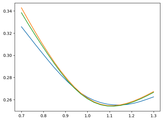
[11]:
nk = 21
k = np.linspace(0.7,1.3,nk)
ivm = torch.zeros(nk)
ivq = torch.zeros(nk)
ivh = torch.zeros(nk)

for it,ik in enumerate(k):
    pm = torch.mean(torch.maximum(Sm-ik,torch.tensor(0.))).detach().numpy()
    ivm[it] = blackanalytics.impliedvolatility(pm, 1., ik, T)
    pq = torch.mean(torch.maximum(Sq-ik,torch.tensor(0.))).detach().numpy()
    ivq[it] = blackanalytics.impliedvolatility(pq, 1., ik, T)
    ph = heston_option_price(ik, 1., theta.detach().numpy(), kappa.detach().numpy(), theta.detach().numpy(), eta.detach().numpy(), rho.detach().numpy(), T)
    ivh[it] = blackanalytics.impliedvolatility(ph, 1., ik, T)
/home/vscode/.local/lib/python3.11/site-packages/scipy/integrate/_quadpack_py.py:575: ComplexWarning: Casting complex values to real discards the imaginary part
  return _quadpack._qagse(func,a,b,args,full_output,epsabs,epsrel,limit)
[12]:
plt.plot(k,ivm)
plt.plot(k,ivq)
plt.plot(k,ivh)
[12]:
[<matplotlib.lines.Line2D at 0x7f7483548d50>]