Maxsoft and heavyside function approximation

Approximating the maxsoft and heavyside function throuch a \(C^\infty\) function is important to apply adjoint-algorithmic differentiation. Here we are showing an alternative to common literature based on the hyperbolic function

from quant_analytics_torch.analytics import maxsoft
import torch
import matplotlib
from matplotlib import pyplot as plt

The hyperbolic function is defined as \(h(x) = x + \sqrt{1+x^2}\)

x = torch.linspace(-5,5,101)

y = {}
y['max'] = torch.maximum(x,torch.zeros(101))
y['1'] = maxsoft.soft_max_hyperbolic(x,1.)

plt.plot(x,y['max'])
plt.plot(x,y['1'])

[<matplotlib.lines.Line2D at 0x7f330f2109d0>]

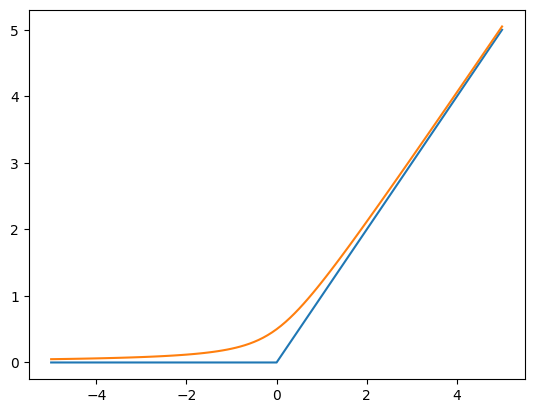
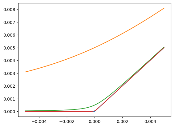
The function closely mimicks \(f(x)=\max\left(x,0\right)\). Adding a scaling parameter \(\epsilon\) allows to vary the degree of approximation via \(h_\epsilon(x) = h(x / \epsilon) \cdot \epsilon\). Below illustrates this for a smaller x-interval

x = torch.linspace(-0.005,0.005,101)
y = {}
y['max'] = torch.maximum(x,torch.zeros(101))
y['0.01'] = maxsoft.soft_max_hyperbolic(x,0.01)
y['0.001'] = maxsoft.soft_max_hyperbolic(x,0.001)
y['0.0001'] = maxsoft.soft_max_hyperbolic(x,0.0001)

plt.plot(x,y['max'])
plt.plot(x,y['0.01'])
plt.plot(x,y['0.001'])
plt.plot(x,y['0.0001'])

[<matplotlib.lines.Line2D at 0x7f330f0f8310>]

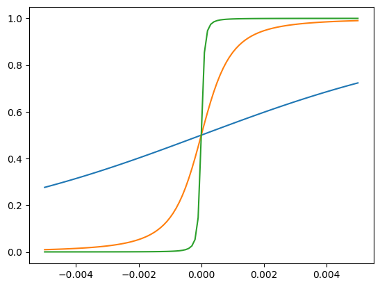
This also allows to approximate the heavisde function \(1_{\{x>0\}}=f^\prime(x)\), through \(h^\prime(x)=\frac 12 + \frac{x}{2\sqrt{1+x^2}}\)

z = {}
z['0.01'] = maxsoft.soft_heavy_side_hyperbolic(x,0.01)
z['0.001'] = maxsoft.soft_heavy_side_hyperbolic(x,0.001)
z['0.0001'] = maxsoft.soft_heavy_side_hyperbolic(x,0.0001)

plt.plot(x,z['0.01'])
plt.plot(x,z['0.001'])
plt.plot(x,z['0.0001'])

[<matplotlib.lines.Line2D at 0x7f330cf75510>]